Creating normal maps from diffuse maps

When I looked around the inter-webs to see how people go about doing this, pretty much everybody and their grandmother was talking about using a Sobel filter as the one and only true way.

An apparent general consensus about any subject, will always make me suspicious and curious about exploring alternative ways of doing said thing.

Before we get started, let’s pick a suitable test subject in the form of a rather lovely and hand-painted 512x512 stone floor texture from opengameart.org.

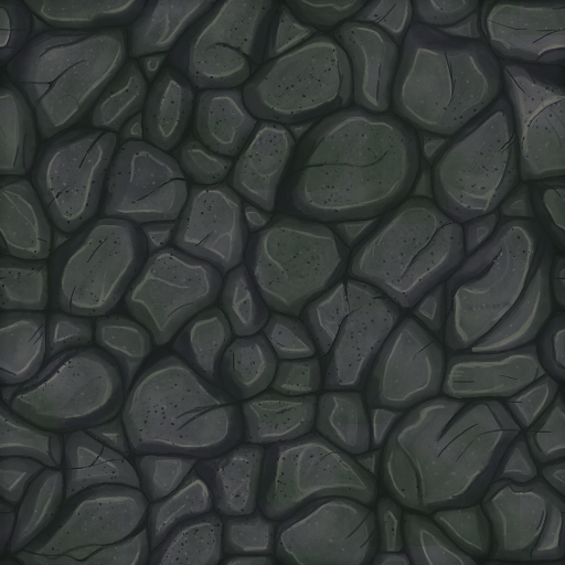
The first order of business is to turn the diffuse map into a height-map by converting every pixel into its gray-scale equivalent.

/*
	MIT LICENSE
	Copyright (c) 2023, Mihail Szabolcs
*/
typedef union
{
    uint32_t opaque;
    struct
    {
        uint32_t r : 8;
       	uint32_t g : 8;
        uint32_t b : 8;
        uint32_t a : 8;
    };
} rgba_t;

void build_normal_map(const rgba_t *input, rgba_t *output, int w, int h)
{
    int x, y;
    uint32_t gray;
    rgba_t c;

    for(y = 0; y < h; y++)
    {
        for(x = 0; x < w; x++)
        {
            c = input[x + y * w];
            gray = (c.r + c.g + c.b) / 3.0f;

            c.r = gray;
            c.g = gray;
            c.b = gray;

            output[x + y * w] = c;
        }
    }
}

We do this by calculating the average of the r, g and b components of every pixel, which results in an image like the one presented below. Nothing too fancy or ground breaking.

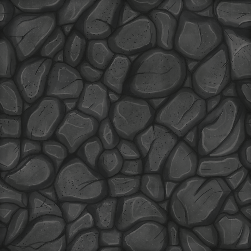
Of course that we could use some other formula to convert to gray-scale, rather than just taking the average, but this is more than good enough for our purposes.

Now it is time to turn the height-map into a normal-map (bump map) by calculating the change in height for every pixel in the input height-map and storing the result in the output normal map.

To do this, we simply sample 4 pixels around the current pixel, calculate the difference on the x and y axis respectively and then “normalize” the value from the [-1, 1] range to [0, 1] and then finally [0, 255] range.

We also invert the green channel, which holds the value of the Y axis, because we intend to use the normal map with OpenGL. In case of DirectX, this is [unnecessary][invertgreenchannel]. Obviously, this could also be inverted at run-time when the normal map is loaded or in a shader.

/*
	MIT LICENSE
	Copyright (c) 2023, Mihail Szabolcs
*/
#define minf(a, b) ((a) < (b) ? (a) : (b))
#define maxf(a, b) ((a) > (b) ? (a) : (b))
#define grayscalef(c) ((c.r + c.g + c.b) / 3.0f)

void build_normal_map(const rgba_t *input, rgba_t *output, int w, int h)
{
    int x, y;
    float gu, gd, gl, gr, dx, dy;
    rgba_t c;

    for(y = 0; y < h; y++)
    {
        for(x = 0; x < w; x++)
        {
            gu = grayscalef(input[x + maxf(y - 1, 0) * w]);
            gd = grayscalef(input[x + minf(y + 1, h - 1) * w]);
            gl = grayscalef(input[maxf(x - 1, 0) + y * w]);
            gr = grayscalef(input[minf(x + 1, w - 1) + y * w]);

            dx = (gl - gr) / 255.0f * 0.5f + 0.5f;
            dy = (gu - gd) / 255.0f * 0.5f + 0.5f;

            c = input[x + y * w];
            c.r = dx * 255;
            c.g = 255 - dy * 255;
            c.b = 255;

            output[x + y * w] = c;
        }
    }
}

The result is a little bit anemic to say the least, but it’s still possible to see some of the bevels if one squints just the right way. At any rate, this is not very promising at all, but it’s more than nothing.

Let’s take a look at what we could do in order to improve this situation. If we load up the resulting normal map in GIMP and then play around with the “Curves” tool, we can notice that an S-shaped curve seems to help quite bit.

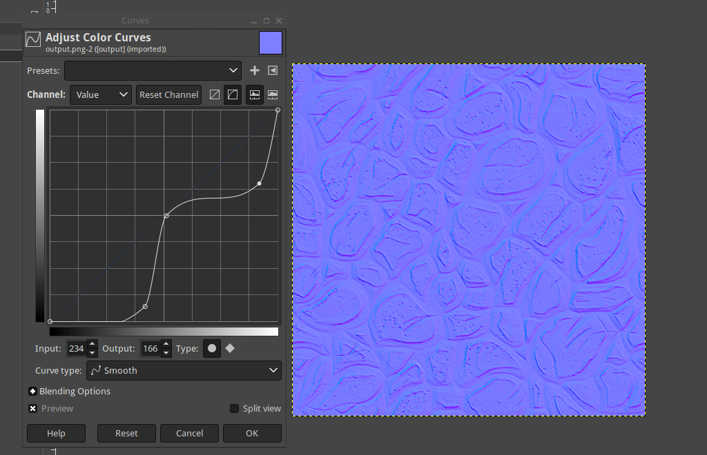
We could just use a Bezier curve with 2 control points and interpolate to achieve a similar curve, but there’s another way by making good use of a so called sigmoid curve.

Let’s head over to the desmos graphing calculator and plot this very cute sigmoid curve.

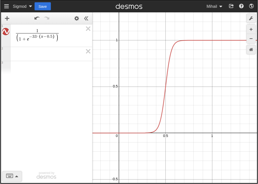
The -33 is simply a magic number that is good enough and was chosen purely arbitrarily. If we were to turn this into an actual tool, then we would probably also want to make this a user configurable as it can affect the output in various ways.

We also shift the curve to the right by 0.5 hence the x - 0.5.

/*
	MIT LICENSE
	Copyright (c) 2023, Mihail Szabolcs
*/
void build_normal_map(const rgba_t *input, rgba_t *output, int w, int h)
{
    int x, y;
    float gu, gd, gl, gr, dx, dy;
    rgba_t c;

    for(y = 0; y < h; y++)
    {
        for(x = 0; x < w; x++)
        {
            gu = grayscalef(input[x + maxf(y - 1, 0) * w]);
            gd = grayscalef(input[x + minf(y + 1, h - 1) * w]);
            gl = grayscalef(input[maxf(x - 1, 0) + y * w]);
            gr = grayscalef(input[minf(x + 1, w - 1) + y * w]);

            dx = (gl - gr) / 255.0f * 0.5f + 0.5f;
            dy = (gu - gd) / 255.0f * 0.5f + 0.5f;

            dx = 1.0f / (1.0f + exp(-33 * (dx - 0.5f)));
            dy = 1.0f / (1.0f + exp(-33 * (dy - 0.5f)));

            c = input[x + y * w];
            c.r = dx * 255;
            c.g = 255 - dy * 255;
            c.b = 255;

            output[x + y * w] = c;
        }
    }
}

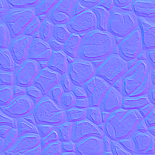
Quite an improvement compared to what we got before, with many of the finer details now coming through as one would expect. Now let’s do some optimizations before we wrap this all up and call it a day.

It turns out that we can do away with most of the divisions by multiplying with the inverse and pre-calculate some of the index offsets on the y axis which lets us avoid some of the useless multiplications that we are currently doing when calculating the actual index into the input and the output arrays.

/*
	MIT LICENSE
	Copyright (c) 2023, Mihail Szabolcs
*/
#define GRAYSCALE_INV (1.0f / (3.0f * 255.0f))
#define grayscalef(c) ((c.r + c.g + c.b) * GRAYSCALE_INV)

void build_normal_map(const rgba_t *input, rgba_t *output, int w, int h)
{
    int x, y, ww, hh, yo, you, yod;
    float gu, gd, gl, gr, dx, dy;
    rgba_t c;

    ww = w - 1;
    hh = h - 1;

    for(y = 0; y < h; y++)
    {
       	yo = y * w;
        you = maxf(y - 1, 0) * w;
        yod = minf(y + 1, hh) * w;

        for(x = 0; x < w; x++)
        {
            gu = grayscalef(input[x + you]);
            gd = grayscalef(input[x + yod]);
            gl = grayscalef(input[maxf(x - 1, 0) + yo]);
            gr = grayscalef(input[minf(x + 1, ww) + yo]);

            dx = (gl - gr) * 0.5f + 0.5f;
            dy = (gu - gd) * 0.5f + 0.5f;

            dx = 1.0f / (1.0f + exp(-33 * (dx - 0.5f)));
            dy = 1.0f / (1.0f + exp(-33 * (dy - 0.5f)));

            c = input[x + yo];
            c.r = dx * 255;
            c.g = 255 - dy * 255;
            c.b = 255;

            output[x + yo] = c;
        }
    }
}

We could have also gotten rid of the clamping if we wanted to by simply doing a bitwise modulo on the x and y variables; this assumes that the width and height are power of two in which case we know that the following is true:

x & (w - 1) = x % w
y & (h - 1) = y % h

Yet another thing we could have done is to add the restrict qualifier to the input and output arguments in order to give an extra hint to the compiler that input and output arrays never actually overlap.

static void build_normal_map(
    const rgba_t *restrict input,
    rgba_t *restrict output,
    int w,
    int h
)

If your C compiler of choice supports C11, then restrict should be available, if not, then it might still be available under a different name like __restrict.

And now, let us take a final look at our handy work by checking out the resulting normal map in action with one rotating light source.

Not too shabby, right? I think so too as well.